[Write to Learn Series] You May Not Know Linear Regression Enough! Discover the Causal Effect of Credit Limit on Risk
![[Write to Learn Series] You May Not Know Linear Regression Enough! Discover the Causal Effect of Credit Limit on Risk](/content/images/size/w1200/2023/12/ci.png)
Disclaimer: The accuracy of the information in this article is not guaranteed. The methodologies discussed are conceptual and not yet implemented in business.
A common challenge in consumer loan industries is balancing risk management with credit limit increases. Credit limits, often determined by expert judgment, are typically excluded from the Behavior Scorecard Model (B-Score) to maintain prediction stability. Traditional machine learning models struggle with changes in feature distributions and may inaccurately portray the relationship between credit limits and risk. This phenomenon was particularly evident in my analysis of the Brazil market, which exhibits a stronger sensitivity to credit limits compared to Southeast Asian markets I've worked in (ID, PH, VN, MY).
In Brazil, I hypothesize – though unvalidated – that the high household debt ratio, compounded by elevated interest rates, makes consumers more susceptible to debt. This contrasts with Southeast Asia, where credit limits haven't reached a risk tipping point. This insight underscores the need to understand the nuanced relationship between credit limits and risk, identifying features that differentiate user sensitivity.
The standard approach involves hypothesis-driven experiments, such as segmenting users by income for randomized controlled trials (RCTs). However, the complexity and duration of such tests, along with their exponential increase in dimensionality and resource requirements, limit their feasibility. An alternative is universal testing, but this is cost-prohibitive in the credit industry due to the randomness of credit limit assignments.
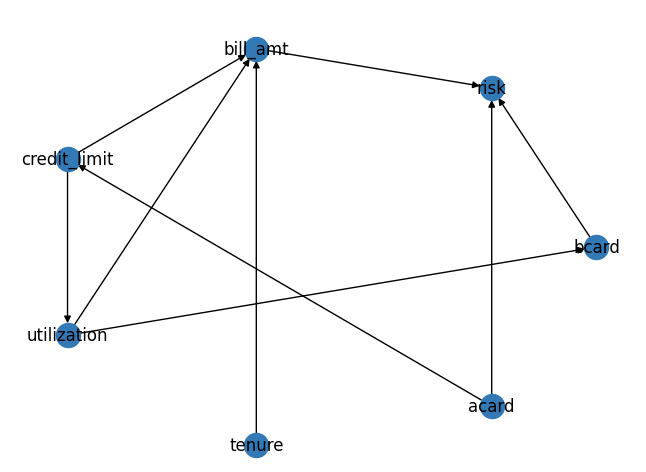
To circumvent these challenges, we can explore the treatment effect by assuming a causal mechanism between credit limits and risk. Let's consider six variables: Application Scorecard (Acard), Behavior Scorecard (Bcard), utilization, tenure, credit limit, and bill amount. These are represented in a Direct Acyclic Graph (DAG), illustrating their causal relationships.


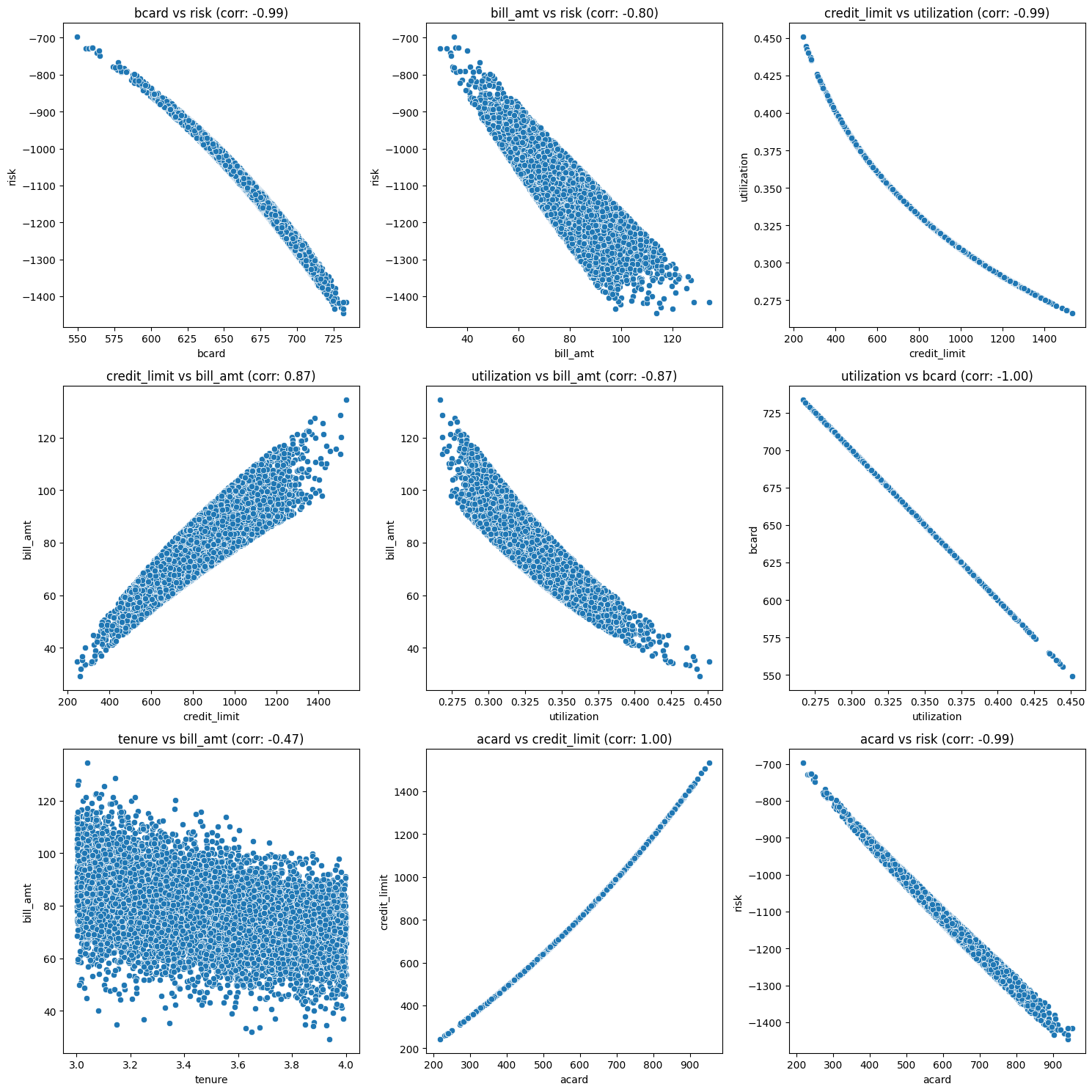
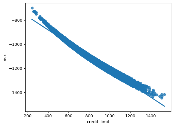
By generating synthetic data based on this DAG, we observe a negative correlation between risk and credit limit. However, this is confounded by Acard's influence on both variables.
sns.regplot(x=synthetic_data_v2['credit_limit'],y=synthetic_data_v2['risk'])

The influence of Acard on both Credit Limit and Risk is pivotal: higher Acard scores often lead to increased credit limits, and conversely, a higher Acard typically indicates lower risk. This makes Acard a key confounder (in the pattern B<--A-->C, A is the confounder). Experienced analysts are adept at controlling for Acard to draw accurate conclusions. However, the addition of more variables can complicate the analysis. Take, for instance, the observation that higher bill amounts correlate with lower risk. Intuitively, one might expect the opposite since a larger bill amount suggests a greater repayment burden, presumably increasing risk. A closer look at the Direct Acyclic Graph (DAG) reveals that the confounding factors here are the interactions between Acard/Credit Limit and Bcard/Utilization. By appropriately adjusting for these confounders, we can uncover positive correlations that align more closely with our intuitive understanding of these relationships.
How are all these related to Linear Regression? The answer lies in The Frisch-Waugh-Lowell Theorem (FWL). Controlling for confounders is equivalent to adding the confounders to the regression.
smf.ols('risk ~ credit_limit + acard', synthetic_data_v2).fit().summary().tables[1]
coef | std err | t | P>|t| | [0.025 | 0.975] | |
|---|---|---|---|---|---|---|
| Intercept | -472.3541 | 2.883 | -163.844 | 0.000 | -478.005 | -466.703 |
| credit_limit | 0.1993 | 0.012 | 17.136 | 0.000 | 0.177 | 0.222 |
| acard | -1.3416 | 0.021 | -65.396 | 0.000 | -1.382 | -1.301 |
credit limit is now positively correlated to risk.
smf.ols('risk ~ bill_amt + utilization + acard', synthetic_data_v2).fit().summary().tables[1]
coef | std err | t | P>|t| | [0.025 | 0.975] | |
|---|---|---|---|---|---|---|
| Intercept | -1000.0000 | 3.27e-12 | -3.06e+14 | 0.000 | -1000.000 | -1000.000 |
| bill_amt | 2.0000 | 2.49e-15 | 8.03e+14 | 0.000 | 2.000 | 2.000 |
| utilization | 1000.0000 | 7.04e-12 | 1.42e+14 | 0.000 | 1000.000 | 1000.000 |
| acard | -1.0000 | 1.6e-15 | -6.26e+14 | 0.000 | -1.000 | -1.000 |
bill amt is now positively correlated to risk.
The FWL Theorem states that the following are equivalent:
- the OLS estimator obtained by regressing y on x₁ and x₂
- the OLS estimator obtained by regressing y on x̃₁, where x̃₁ is the residual from the regression of x₁ on x₂
The second method says that the residuals from this regression represent the part of X1 that is independent of the other variables. Then, the final regression estimates the relationship of y on x1 free from the impact of other variables.
Could I control all variables then? Let's try:
smf.ols('risk ~ credit_limit + acard + utilization + bill_amt + tenure', synthetic_data_v2).fit().summary().tables[1]
| Intercept | -1000.0000 | 1.56e-10 | -6.39e+12 | 0.000 | -1000.000 | -1000.000 |
|---|---|---|---|---|---|---|
| credit_limit | -7.827e-15 | 6.23e-14 | -0.126 | 0.900 | -1.3e-13 | 1.14e-13 |
| acard | -1.0000 | 1.76e-13 | -5.67e+12 | 0.000 | -1.000 | -1.000 |
| utilization | 1000.0000 | 3.03e-10 | 3.3e+12 | 0.000 | 1000.000 | 1000.000 |
| bill_amt | 2.0000 | 1.71e-13 | 1.17e+13 | 0.000 | 2.000 | 2.000 |
| tenure | -3.212e-12 | 3.84e-12 | -0.837 | 0.403 | -1.07e-11 | 4.31e-12 |
There is no relationship between credit limit and risk. We need to select the right variables to be included in the regression.
This method enables us to explore credit limit and risk relationships without extensive RCTs, allowing for more efficient user segmentation and feature testing, which I will try to cover in the next post on Effect Heterogeneity.
However, it's crucial to remember that causal diagrams are based on assumptions that may not always hold. They can be challenged and refined using real-world data and analytical techniques like d-separation or conditional independence testing.
For an in-depth exploration and practical application of these concepts, feel free to visit the accompanying Google Colab notebook: https://colab.research.google.com/drive/1KeQUkB2eiHKTgT_2S_rr8trbZv-lbGUX?usp=sharing


Comments ()