[Write to Learn] How Exploring Can Increase Long-Term Reward? An Illustration Using Epsilon-Greedy Method.

The example presented in Reinforcement Learning: An Introduction by Sutton and Barto. A possible value added by this article is to provide a more detailed explanation and code snippets to replicate the example.

The 10-armed Bandit Example

For readers not familiar with the k-armed bandit problem, you are repeatedly faced with a choice among k different options, and your objective is to maximise the expected total reward. It is called a bandit because it is an analogy to a slot machine or "one-armed bandit".

Imagine a 10-armed bandit where the reward of selecting \(a\), \(q_*(a)\), was chosen according to a normal distribution with mean zero and unit variance. The actual reward of \(q_*(a)\) was selected from a normal distribution with mean zero and unit variance. Simply put, the mean reward of choosing different options (1,2, ...,10) is a standard normal distribution. The actual reward received also varies around the mean, following a standard normal distribution.

import numpy as np
import matplotlib.pyplot as plt

# Number of actions
num_actions = 10

# Means of the reward distributions for each action, drawn from a standard normal distribution
means = np.random.normal(0, 1, num_actions)

# Variance of the reward distributions
variance = 1

# Draw samples from normal distributions centered around the means for each action
actions = np.arange(1, num_actions + 1)  # Actions labeled from 1 to 10

# Plotting the reward distributions as violin plots
data = [np.random.normal(m, variance, 2000) for m in means]
plt.violinplot(data, actions, widths=0.9, showmeans=True)

# Adding labels and title
plt.xlabel('Action')
plt.ylabel('Reward distribution')
plt.title('10-armed bandit problem - Reward distribution')

# Annotate the means for each action
for i, mean in enumerate(means):
    plt.text(i+1.1, mean, f'q*({i+1})', horizontalalignment='center', color='black')

plt.show()

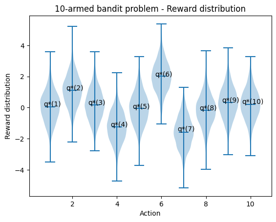
Given these reward distributions, we develop an algorithm that maximises the long-term reward over 1000 steps.

Epsilon-Greedy Method Implementation

Initially, the agent does not know the reward of each action because, if so, the agent can always select the action with the highest reward. \(Q(a)\) is the estimated reward of action \(a\). \(N(a)\) is the number of times action \(a\) is chosen. \(R\) is the reward. You may be confused about capital letters and lowercase letters. In the Summary of Notation session of the book, the author explains that capital letters are used for random variables. In contrast, lowercase letters are used for values of random variables and scalar functions. To understand the below algorithm, I find it unnecessary to bother with this detail.

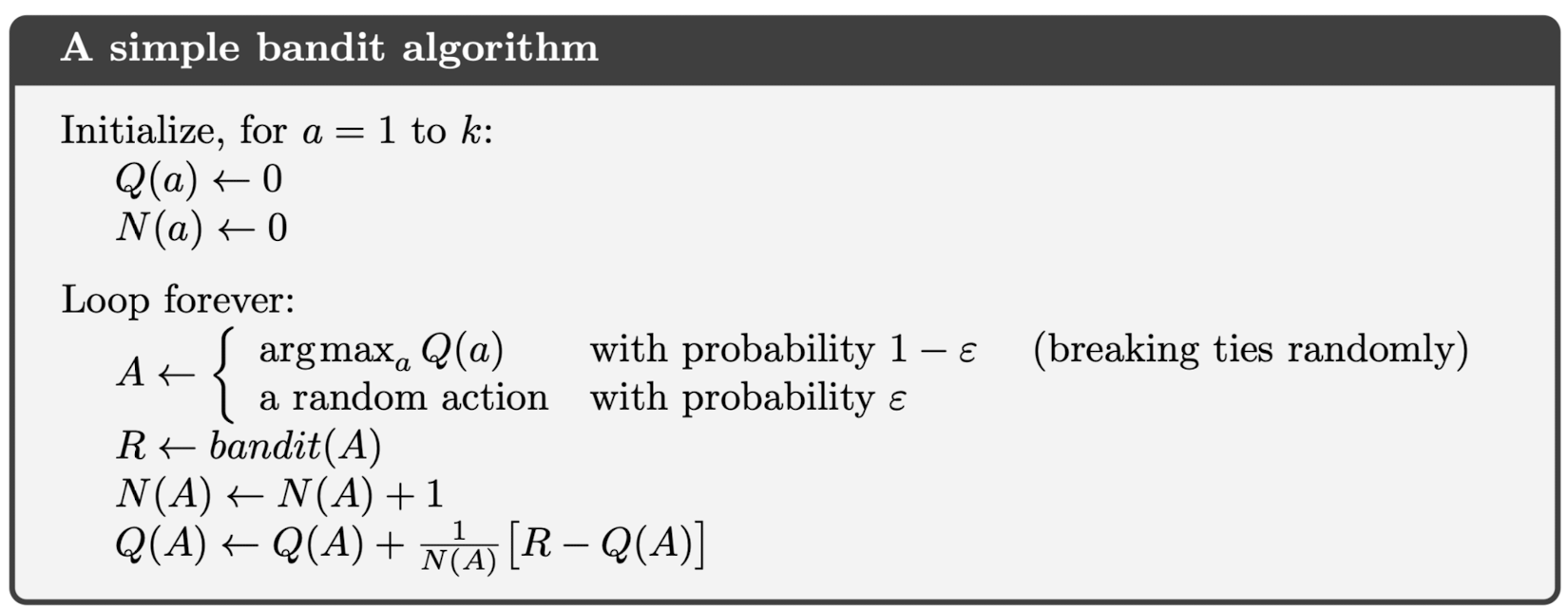
To begin with, we initiated the value and counter of each action to be zero. If we want to be greedy, we will always exploit current knowledge to maximise immediate reward. Then \(A \leftarrow argmax_a Q(a)\). It spends no time sampling other actions that might be better than all previous experiences. A simple alternative is to behave naively for an "epsilon" amount of time. Then, we compute the reward based on the distribution we assumed.

Finally, we have to update the value of the action taken based on the feedback from the environment and increase the counter by one. The last formula can be understood as a recursion.

\[\begin{align} Q_{n+1} &= \frac{1}{n}\sum_{i=1}^{n} R_i \\ &= \frac{1}{n} \left( R_n + \sum_{i=1}^{n-1} R_i \right) \\ &= \frac{1}{n} \left( R_n + (n - 1)\frac{1}{n - 1}\sum_{i=1}^{n-1} R_i \right) \\ &= \frac{1}{n} \left( R_n + (n - 1)Q_n \right) \\ &= \frac{1}{n} \left( R_n + nQ_n - Q_n \right) \\ &= Q_n + \frac{1}{n} \left[ R_n - Q_n \right] \end{align}\]

Readers may be confused about why the subscript is \(n+1\) but not \(n\) in equation 1. The new estimated value is based on all previous realised rewards. Equation 6 says that the latest estimate equals the old estimate plus the error in the estimate. The error is the deviation of the latest realised reward from the estimated reward reduced by \(n\) fraction to accurately represent (scale down) the impact of the new estimate.

def run_epsilon_greedy(epsilon, num_actions, steps, data):
    Q = {i: 0 for i in range(1, num_actions + 1)} # a dictionary with action as key and reward as value
    N = {i: 0 for i in range(1, num_actions + 1)} # a dictionary with action as key and counter as value
    total_reward = 0
    average_reward_over_time = [] # total reward divided by step
    
    for step in range(1, steps + 1):
        random_number = random.random()
        if random_number < 1 - epsilon:  # Greedy action
            max_value = max(Q.values())
            A = random.choice([key for key, value in Q.items() if value == max_value])
        else:  # Exploration action
            A = random.choice(list(Q.keys()))

        R = random.choice(data[A - 1])  # Sampling the reward
        N[A] += 1
        Q[A] += 1 / N[A] * (R - Q[A])  # Updating the estimate
        total_reward += R
        average_reward_over_time.append(total_reward / step)
    
    return average_reward_over_time

At first, I thought I had completed it. However, I found that the result can be quite different when I rerun the code. The author mentioned how he got the graph: "For any learning method, we can measure its performance and behaviour as it improves with experience over 1000 time steps when applied to one of the bandit problems. This makes up one run. Repeated this for 2000 independent runs, each with a different bandit problem, we obtained measures of the learning algorithm's average behaviour." However, this also hints that initial configuration can affect the model performance.

def average_runs_optimized(epsilons, num_actions, steps, runs, data):
    average_results = {epsilon: np.zeros(steps) for epsilon in epsilons}
    
    for _ in range(runs):
        for epsilon in epsilons:
            rewards = run_epsilon_greedy(epsilon, num_actions, steps, data)
            average_results[epsilon] += np.array(rewards)
    
    # Averaging the results
    for epsilon in epsilons:
        average_results[epsilon] /= runs
    
    return average_results

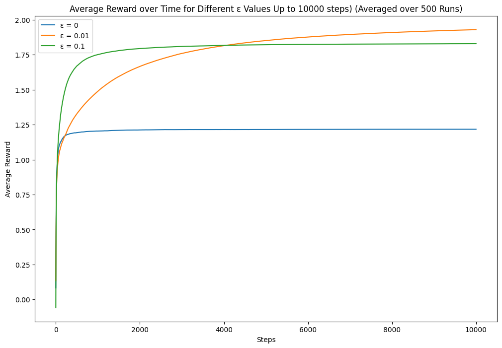
Here is the average result:

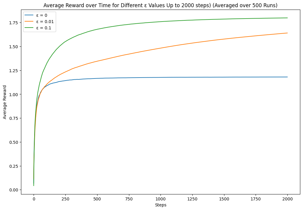
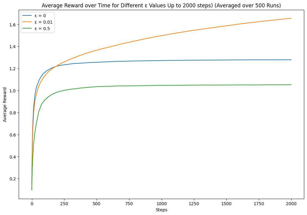
The near-greedy option performs better. Let's try some other combinations. If we increase the epsilon, will it explore too many suboptimal options? If we increase the step size, will it explore too much after the certainty increases?

Takeaways

Exploration can lead to higher long-term rewards, allowing the agent to discover potentially better options. However, too much exploration can be detrimental, preventing the agent from exploiting known, high-reward actions. Finding the right balance is key to maximising rewards. Also, initial configuration can affect the model performance, which is a bias.

Complete code can be found here.