How to Determine the Sample Size of AB Test?

TLDR

For two groups with a two-sided alternative, normal distribution with homogeneous variances ( \(\sigma_0^2 = \sigma_1 ^2 = \sigma ^2)\) and equal sample sizes (\(n_0 = n_1 = n\)),

\[n = \frac{16}{\Delta^2}\]
where
\[\Delta = \frac{\mu_0 - \mu_1}{\sigma} = \frac{\delta}{\sigma}\]

Examples:
What sample size is required if the baseline conversion rate is 2% and the minimal detectable difference is 0.5%?

We need the variance to solve for the sample size using the above equation. Since conversion is just a binomial proportion, the variance is given by \(p \cdot (1-p) \). Then, \[n = \frac{16 \cdot 0.02 \cdot (1-0.02)}{0.005^2} = 12544\] (If you need a refresh on the variance of the binomial distribution, follow this link.)

I know most of you are not satisfied with the conclusion without explanation.

Statistics 101

Before we delve into the sample size calculations, these are the key concepts to understand. If you need a refresher, I have linked to some resources you may find helpful.

• Type I Error (\(\alpha\) or p-value): The probability of rejecting the null hypothesis when true.
• Type II Error (\(\beta\)): The probability of not rejecting the null hypothesis when it is false
• Power \(= 1- \beta\): The probability of rejecting the null hypothesis when it is false.
• \(n, \sigma, \mu, S.E. \): sample size, variance, mean (I find Section 2.4 of the book Introduction to Probability. by Dimitri P. Bertsekas and John N. Tsitsiklis an excellent resource on these topics) , standard error.
• Critical value (\(z\)): The number of standard deviations required to reject the null hypothesis when true. It is closely related to p-value/ confidence intervals.

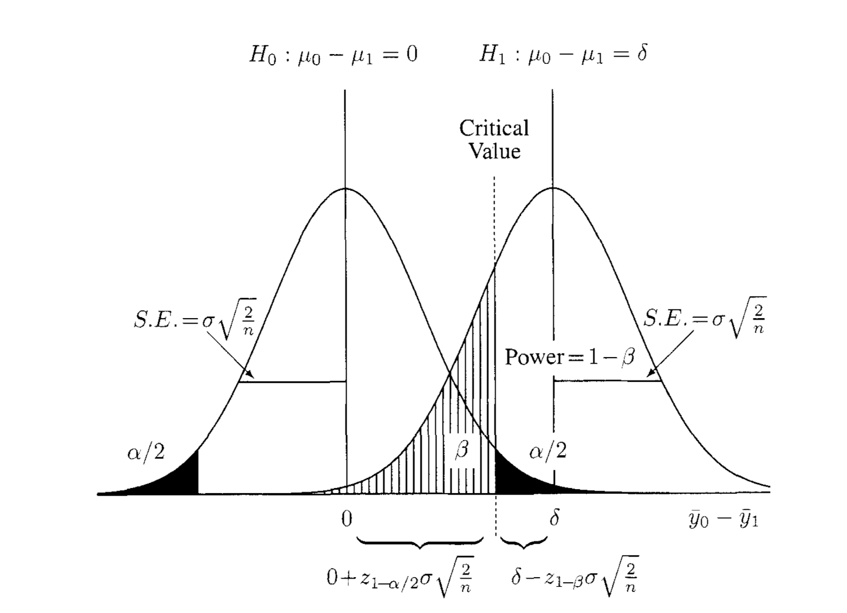
All the statistical concepts you will need to know can be summarised into one graph:

Assuming \(H_0\), the null hypothesis is true, i.e., we sampled from the \(H_0\) distribution, and the p-value represents the probability of observing what you have observed. Because we said if the probability falls within the dark area, we will reject the null hypothesis, that's a false rejection. Thus, the dark area is also a type I error (false negative). Assuming, on the contrary, \(H_1\), the alternative hypothesis is true, i.e., we sampled from the \(H_1\) distribution, the shaped area represents the probability of not rejecting the \(H_0\) given \(\alpha\) because the p-value is less than \(\alpha\). Thus, the shaped area is a type II error (false positive). There is a trade-off between Type I error and Type II error. If we lower one, the other will increase (Imagine moving the critical value line left and right).

The only concept left in this chart at this point is \(S.E.\). Given that we knew the variance, \(\sigma\), of the distribution, the sampling error from \(n\) samples is \(\sigma/n\). The proof can be found on the Wikipedia page. The \(S.E.\) for two samples assuming equal variance (comparing the distribution between \(H_0\) and \(H_1\)) is \(SE = \sqrt{\frac{\sigma^2}{n_1} + \frac{\sigma^2}{n_2}} = \sigma\sqrt{2/n}\). I will not derive the formula here. The derivation used the definition of variance and pooled variance.

Deriving the Sample Size Formula

The critical value defines the boundary between the rejection and nonrejection region. This value must be the same under the null and alternative hypotheses. Thus, the fundamental equation for the two-sample situation: \[0 + z_{1-\alpha/2} \sigma \sqrt{\frac{2}{n}} = \delta - z_{1-\beta} \sigma \sqrt{\frac{2}{n}} \], rearranging it will yield \[n = \frac{2( z_{1-\alpha/2} + z_{1-\beta})^2}{(\frac{\delta}{\sigma}) ^2}\]. For \(\alpha = 0.05\) and \(\beta=0.2\) the values of \(z_{1-\alpha/2}\) and \(z_{1-\beta}\) are 1.96 and 0.84, respectively. So, \(2( z_{1-\alpha/2} + z_{1-\beta})^2 \approx 16\) (You can find the corresponding value in Z-table. Usually, the table is given, but if you are interested in how it is derived, you may refer to this.).

The equation can calculate detectable differences for a given sample size \(n\): \[\delta = \frac{4\sigma}{\sqrt{n}}\]

Q&A

• What if there are more than two groups? The required sample size per group is the same, provided you only compare with the control.
• Is normality a poor assumption? While the sample distribution of the metric \(Y\) does not follow a normal distribution, the average \(\bar{Y}\) usually does because of the Central Limit Theorem.
• Can we stop the experiment once the significant level is reached? NO! The sample size should be predetermined. More detailed explanation here.
• Is there a problem if the metric unit differs from the randomisation unit? Yes. For example, click-through rate (CTR) is the ratio of total clicks to pageviews. The analysis unit is no longer a user but a pageview. When the unit of a user randomises the experiment, this can create a challenge for estimating variance because the assumption is that the samples need to be i.i.d. One trick is to write the ratio metric as the ratio of "average of user level metrics", for example, clicks per user divided by pageviews per user.